Tutorial 1: GAT walkthrough

Abigail Stamm

2023-03-15

Introduction

This vignette is designed for a user with no experience in R who just wants to run the default version of the Geographic Aggregation Tool (GAT). This manual breaks down the different parts of GAT and describes what to do and what to expect using 2010 Census shapefiles for Hamilton and Fulton Counties in New York State, which are embedded in the package. These shapefiles will be used in this manual.

Note: For users who wish to modify GAT, developer options have been written into several of the package functions. Check the functions’ help pages (linked from function names) and the Technical Notes for more information. Users interested only in running GAT can ignore these links.

Objective

This tutorial will walk you through the following activities. You will start with a shapefile of towns in two New York State counties. You will aggregate these towns to a minimum population of 5000 based on population weighted centroids, which will be calculated using census block files.

The results will be displayed in the log and as a series of maps in a PDF. The boundaries of the new areas will be saved as an ESRI shapefile and, if desired, as a Google Earth KML file so that you can import them to your preferred GIS application.

You will also learn the following:

• how to exclude certain areas from aggregation
• how to calculate population density for the aggregated areas

Running GAT

Please note that R is case sensitive. The provided code is designed to be copy-pasted, but if you prefer to type it yourself, be aware of capitalization.

To follow this vignette, you can use the embedded shapefiles in this package. The filepath after the command below points to the folder in your package install that contains these shapefiles. When prompted to select a shapefile, navigate to this filepath.

paste0(tools::getVignetteInfo("gatpkg", all = TRUE)[1, "Dir"], "/extdata/")

Alternatively, you can use your file manager’s search feature to locate the file “hftown.shp”.

To run GAT, you only need one line of code:

gatpkg::runGATprogram()

The steps below will walk you through the dialogs created by GAT and describe the types of input expected using the embedded shapefiles.

GAT starts by creating initial variables and displaying a progress bar that will continually update as it runs. GAT’s processes occur in this order:

• request information in 11 user input steps
• process and aggregate the shapefile
• draw 4 to 7 maps
• save 11 or 12 files

User input section

This is the interactive portion of GAT. The steps below will walk you through what to expect from GAT. If any portion of this section is cancelled, GAT will quit.

GAT starts with this progress bar, which will update as GAT proceeds:

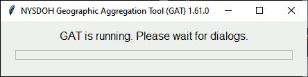
Initial Progress Bar

Do not close the progress bar before GAT finishes running. If you do, GAT will crash with this error:

warning(‘Error in structure(.External(.C_dotTclObjv, objv), class = “tclObj”) :
[tcl] bad window path name “.113”.’)

Step 1. Request aggregation shapefile

This step requests the shapefile from the user using a pop-up dialog. This progress bar will be displayed:

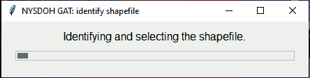
Progress Bar: Identify Shapefile

How this step works

In this dialog, you can navigate to any shapefile on your computer or network. To follow the steps as shown, navigate to the “extdata” folder in your installation of “gatpkg”, which you can reach via your filepath in Running GAT. Select the “hftown” shapefile.

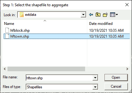
Dialog: Identify Shapefile

Select “hftown.shp” and click Open to move to the next step or click Cancel to end GAT.

About this step

The function locateGATshapefile() checks that:

• the shapefile uses polygons
• at least one character variable can be used as an area identifier (such as name, geoid, or index)
• at least one numeric variable can be aggregated

If any of these checks fail, you will receive an error message and will be asked to select a new shapefile. The “open file” dialog may not look exactly as shown; sometimes it includes a folder list on the left.

Learn more about the example aggregation shapefile, hftown.

Step 2. Request shapefile identifier

This step requests a unique identifier variable from the user using a pop-up dialog. This ID will be overwritten as areas are aggregated and a crosswalk from these identifiers to the ones produced by GAT will be generated at the end.

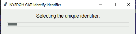
Progress Bar: Identify Identifier

How this step works

In this dialog, select the variable you would like to use from the drop-down list. To follow the steps as shown, select “ID”.

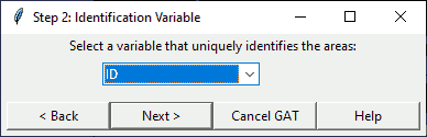
Dialog: Identify Identifier

Click Next > to move to the next step, < Back to move to the previous step (selecting a shapefile), Cancel to end the program, or Help to get further guidance.

About this step

The function identifyGATid() lists only character variables with unique values from the shapefile’s DBF. If the identifier you are looking for does not show up, it may either be numeric or contain at least one non-unique value. If you wish to use a numeric identifier, you will need to convert it to character before running GAT.

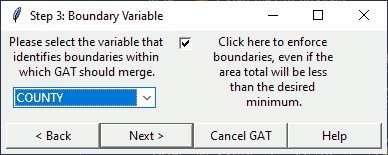
Step 3. Request boundary variable

This step requests the boundary variable from the user using a pop-up dialog. GAT will aggregate within this boundary first, if possible.

Progress Bar: Identify Boundary

How this step works

In this dialog, select the variable you would like to use from the drop-down list. If you would like to require that GAT enforces boundaries, click the checkbox as shown in the image. If you do not want to use a boundary, select “NONE” from the drop-down menu. If you select “NONE”, the program will ignore whether you checked the box.

Dialog: Identify Boundary

To follow the steps as shown, select “COUNTY” and check the box.

Click Next > to move to the next step, < Back to move to the previous step (selecting the identifier), Cancel to end the program, or Help to get further guidance.

About this step

The function identifyGATboundary() lists only character variables with at least one non-unique value from the shapefile’s DBF. If the boundary you are looking for does not show up, it may either be numeric or contain no non-unique values.

Step 4. Request aggregation variables

This step requests the aggregation variables and their desired minimum and maximum values from the user using a pop-up dialog.

Progress Bar: Identify Aggregators

How this step works

In this dialog, select the variables you would like to aggregate from the drop-down lists. Enter your desired minimum and maximum values for each aggregated area in the text boxes. You may want to include minimum values to increase the likelihood of stable rates and a maximum value to either exclude very populous areas or to ensure most areas have roughly the same population size.

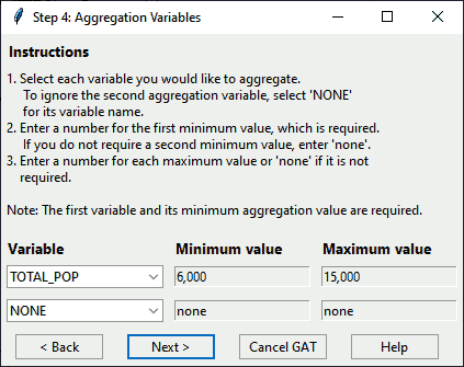
Dialog: Identify Aggregators

To follow the steps as shown, select “TOTAL_POP”. Change the minimum value to “6,000”. Change the maximum value to “15,000”. Leave all options on the second row as “none”.

Click Next > to move to the next step, < Back to move to the previous step (selecting the boundary variable), Cancel to end the program, or Help to get further guidance.

About this step

The function identifyGATaggregators() lists only numeric variables from the shapefile’s DBF. The value boxes can support numbers, commas, and decimals. The value box also allows negative values, but the use of negative values has not been tested in GAT.

If you enter any other characters into the value boxes, you will get an error and a new dialog will appear asking you to re-enter the value. If you enter “none” in the value boxes, that triggers default values, which are the minimum value of the selected variable for “minimum value” and the sum of values for the selected variable for “maximum value”.

Step 5. Request exclusion criteria

This step requests up to three exclusion criteria from the user using a pop-up dialog.

Progress Bar: Identify Exclusions

How this step works

In this dialog, select each variable you would like to use to define exclusions from the drop-down lists. For each variable selected, choose a condition and enter a numeric value. Areas meeting any of these criteria will be removed from the aggregation, but retained in the shapefile. If you do not want to use an exclusion criterion, select “NONE” from the drop-down menu. If you select “NONE”, the program will ignore the corresponding condition and value.

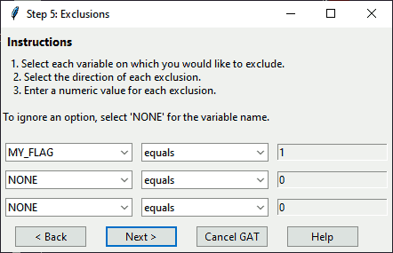
Dialog: Identify Exclusions

To follow the steps as shown, select “MY_FLAG”. Leave the condition as “equals” and change the value to “1”. This will exclude one area to illustrate how excluded areas are displayed on the generated maps and indicated in the generated DBF and log files. Leave the other two criteria as “NONE”.

Click Next > to continue, < Back to move to the previous step (selecting the aggregation variables), Cancel to end the program, or Help to get further guidance.

You will get the following confirmation dialog.

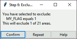
Dialog: Confirm Exclusion Criteria

Click Yes to move to the next step, < Back to move to the previous step (selecting the merge method), Repeat to return to the exclusion criteria, or Help to get further guidance.

About this step

The function inputGATexclusions() lists only numeric variables from the shapefile’s DBF and the option “NONE”. The value dialog can support numbers, commas, and decimals. The value box also allows negative values, but the use of negative values has not been tested in GAT.

You will get an error message and a request to reselect criteria if:

• you enter any characters into the value box other than numbers, comma, decimal, or dash
• you exclude all areas or all except one area

Step 6. Request merge type

This step requests the merge method from the user using a pop-up dialog.

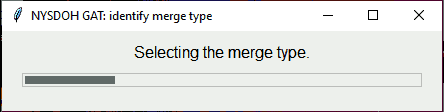
Progress Bar: Identify Merge Type

How this step works

In this dialog, select the method you would like to use to aggregate areas. If you select any option other than “closest area by population-weighted centroid”, geographic centroid will be used. Drop-downs are ignored for options that are not selected.

Dialog: Identify Merge Type

To follow the steps as shown, select “closest area” and choose “population-weighted” from the drop-down.

Click Next > to move to the next step, < Back to move to the previous step (selecting the exclusion criteria), Cancel to end the program, or Help to get further guidance.

About this step

The function inputGATmerge() lists only numeric variables from the shapefile’s DBF for the ratio drop-downs. The ratio denominator (second list) lists only numeric variables without zero or missing values after removing exclusion criteria.

You will get an error message and a request to reselect criteria if:

• you select the same variable for the numerator and denominator when selecting “area with most similar ratio of …”

For more information about the different merge options, including advanced options and how to trigger them, see Selecting the most eligible neighbor in the Technical Notes.

Step 7. Request population shapefile

This step requests the population shapefile from the user using a pop-up dialog. If you select an option other than “closest population-weighted centroid” in the previous dialog, this step is skipped.

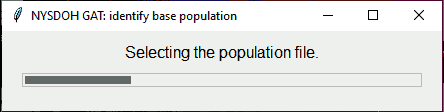
Progress Bar: Identify Population Shapefile

How this step works

In this dialog, you can navigate to any shapefile on your computer or network.

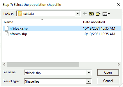
Dialog: Identify Population Shapefile

To follow the steps as shown, navigate to the “extdata” folder in your installation of “gatpkg”, if it does not open automatically. Select the “hfblockgrp” shapefile.

Click “Open” to move to the next step or click “Cancel” to go back to the merge selection dialog.

If there are multiple numeric variables, you will get a dialog requesting that you select one. If there is only one suitable variable, you will get this message:

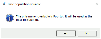
Dialog: Confirm Population Shapefile

Click “Yes” to continue or “No” to return to the previous step (selecting the merge method).

About this step

You can select the same file for both aggregating and population weighting. GAT treats them as two separate objects, so you will still have to identify the population variable for the new object.

The shapefiles’ areas do not need to line up (for example, census tracts within counties) because the population weighting intersects the population object with the aggregation object and assigns population to intersected areas based on the population proportion of each area that falls inside each area to aggregate.

If a population file does not cover the full extent of the areas to aggregate, geographic centroids will be used for areas that cannot be assigned population-weighted coentroids. You will not get a warning if this occurs, so please check your shapefiles before reading them into GAT.

Learn more about the example population shapefile, hfpop.

Step 8. Request rate calculation information

This step requests the rate calculation information from the user using a pop-up dialog.

Progress Bar: Identify Rate Settings

How this step works

In this dialog, select the numerator, denominator, and map color scheme from the drop-downs. Enter a rate name and multiplier value. If you check “Do NOT calculate a rate” at the top, all other options are ignored.

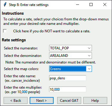
Dialog: Identify Rate Settings

To follow the steps as shown, select “TOTAL_POP” for the numerator, “AREALAND” for the denominator, and “Greens” for the map color scheme. Name your rate variable “pop_dens” (short for “population density”) and leave the multiplier as “10,000”.

Click Next > to move to the next step, < Back to move to the previous step (selecting merge settings), Cancel to end the program, or Help to get further guidance.

About this step

This step is optional. To skip rate calculation, check the box beside “Click here if you do NOT want to calculate a rate.”

The function inputGATrate() lists only numeric variables from the shapefile’s DBF for the numerator and denominator drop-downs. The denominator lists all numeric variables, but can be modified to list only numeric variables without zero or missing values, after removing exclusion criteria.

The rate name must:

• start with a letter or underscore,
• contain only letters, underscores, and numbers, and
• be no longer than 10 characters (the maximum length for DBF variable names; longer names will be truncated).

All characters that are not letters, underscores, or numbers will be removed from the rate name. Do not use the rate name “no_rate”; it is reserved to designate when the rate will not be calculated.

The multiplier box can support numbers, commas, and decimals. If you enter any other characters into the multiplier box, you will get an error and a new dialog will appear asking you to re-enter the multiplier. To calculate a ratio, set the multiplier to 1.

Step 9. Request whether to save KML file

This step asks whether the user wants to save a KML file using a pop-up dialog.

Progress Bar: Save KML

How this step works

In this dialog, select “Yes” or “No”.

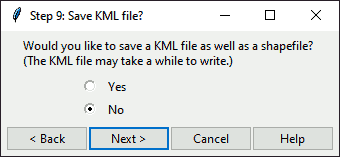
Dialog: Save KML

To follow the steps as shown, select “No”.

Click Next > to move to the next step, < Back to move to the previous step (selecting the rate settings), Cancel to end the program, or Help to get further guidance.

About this step

The function saveGATkml() requests a simple “Yes” or “No”. While a KML file is optional, a shapefile is saved by default.

Step 10. Request where to save shapefile

This step asks the user where to save the shapefile using a pop-up dialog.

Progress Bar: Save File

How this step works

In this dialog, you can navigate to any folder on your computer or network.

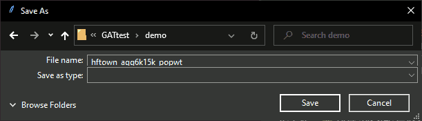
Dialog: Save File

To follow the steps as shown, navigate to your documents folder. Enter “hftown_agg6k15k_popwt”.

Click “Save” to move to the next step or click “Cancel” to end GAT.

About this step

The function saveGATfiles() checks if the name you provide already exists. If so, it asks if you want to overwrite the existing files. All files created will be saved here, with this filename (including log, plots, and KML, if requested).

Step 11. Request settings confirmation

Progress Bar: Confirm GAT Settings

This step requests confirmation of all settings from the user using a pop-up dialog.

How this step works

In this dialog, you can select a step to modify or move on. To modify steps, select the first step you want to modify from top to bottom. After each modification, you will return to this dialog to select the next step.

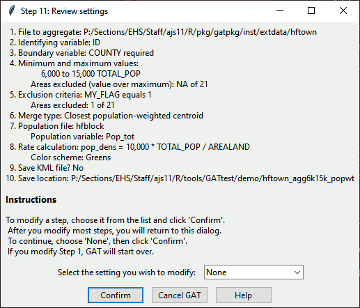
Dialog: Confirm GAT Settings

If you choose to move on, select an item from the drop-down menu and click Confirm. To cancel, click Cancel GAT. Click Help to get further guidance. To follow the steps as shown, select “None” and click Confirm.

About this step

The function confirmGATbystep() requests a simple Yes or No. To end GAT from here, click the “x” in the upper right corner.

Shapefile processing section

At this point, if the user has not cancelled the program, the shapefile processing begins.

Step 12. Read shapefile

Progress Bar: Read the Shapefile

The first processing step is to read in the shapefile. In this step, R creates a simple features object, reads its projection, and calculates the geographic centroid for each polygon. Then GAT creates a flag variable to apply exclusion criteria to relevant polygons based on the exclusions and maximum values that you selected.

About this step

This step was already done in the user input section to assess the shapefile’s suitability for aggregating, but the shapefile was not retained in memory at that point.

Step 13. Run aggregation loop

Progress Bar: Run the Aggregation

This is the second processing step and probably the slowest step in the entire program, especially if you select population weighting. It opens a new progress bar specifically for the aggregation loop. This progress bar updates with the number of areas left to aggregate as each aggregation completes, then closes when the loop finishes.

About this step

This step calls the function defineGATmerge() to create the aggregation key or crosswalk. It creates a subset of polygons for which their value for the aggregation variable(s) is below your minimum desired aggregation value(s). It reorders the subset from largest to smallest aggregation value. Starting with the largest value, it determines acceptable neighbors for aggregation based on your settings.

Step 14. Aggregate areas

Progress Bar: Clean Up the Shapefile

This is the third processing step, which aggregates areas as defined by the crosswalk created in Step 13. If you requested rates, they are calculated in this step.

About this step

This step calls the function mergeGATareas() to perform the aggregation. It also cleans up row names and other information that may not have been properly retained during the aggregation.

Step 15. Calculate compactness ratio

Progress Bar: Calculate GAT Compactness Ratio

This step creates a new compactness ratio variable that is added to the aggregated shapefile’s dataset.

About this step

This step runs the function calculateGATcompactness().

Mapping section

This section contains the maps that are created by GAT. The final PDF will contain between four and seven maps, depending on your selections. Given all seven maps:

• Maps 1 & 2: Choropleths of the first aggregation variable before and after aggregating.
• Maps 3 & 4: Choropleths of the second aggregation variable before and after aggregating (optional).
• Map 5: Comparison of original and aggregated areas.
• Map 6: Choropleth of the compactness ratio after aggregating.
• Map 7: Choropleth of the rate, ratio, or density defined in the rate selection (optional).

Note: R package documentation allows you to view images, but not link to them. For all maps, view larger images by right clicking on the maps and selecting, “Open image in new tab.”

Step 16. Map first aggregation variable

Progress Bar: Map First Aggregation Variable

Two choropleth maps are produced in this step. The two maps use the same color scale and range, which should make comparisons easy.

• Left map: distribution of the aggregation variable before aggregating.
• Right map: distribution of the aggregation variable after aggregating.

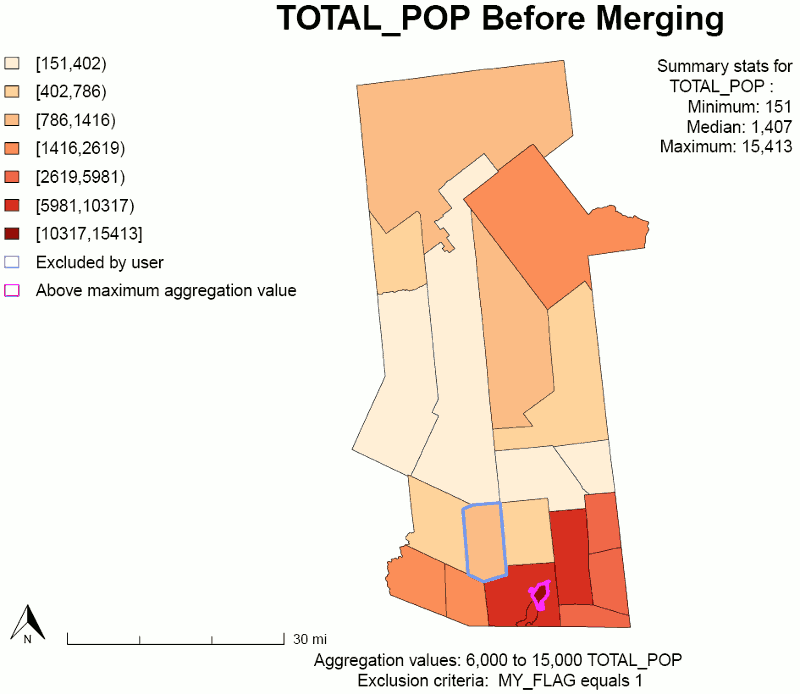
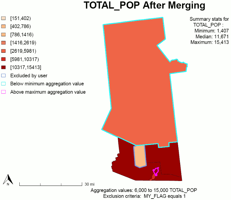
Maps: First Aggregation Variable Before and After Aggregating

About this step

This step calls the function plotGATmaps() to draw the map.

Step 17. Map second aggregation variable

If you selected a second aggregation variable, two choropleth maps are produced in this step. One map shows the distribution of the second aggregation variable before aggregating and the other shows the distribution after aggregating.

About this step

This step calls the function plotGATmaps() to draw the map.

Step 18. Map comparison of old and new areas

Progress Bar: Compare Original and Aggregated Areas

In this map, the aggregated area map is overlaid on top of the original map so you can see how smaller areas combined into larger ones.

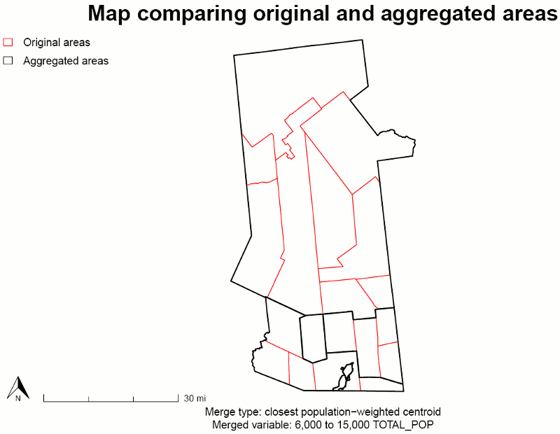
Map: Compare Original and Aggregated Areas

About this step

This step calls the function plotGATcompare() to draw the map.

Step 19. Map compactness ratio

Progress Bar: Map GAT Compactness Ratio

This map displays a choropleth scale of the compactness ratios for the aggregated areas.

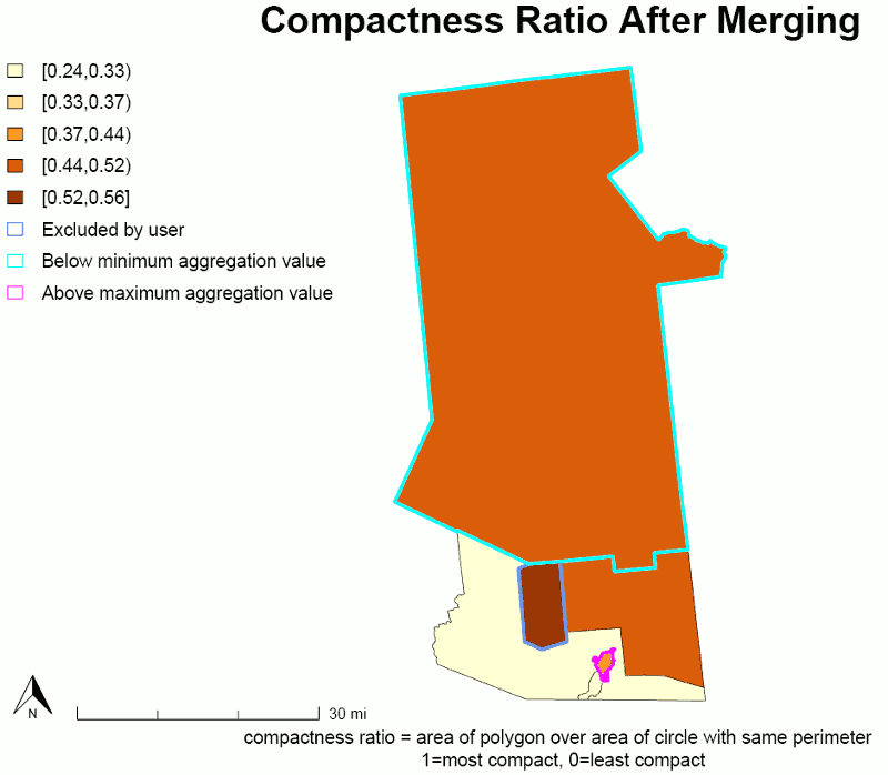
Map: Compactness Ratio

About this step

This step calls the function plotGATmaps() to draw the map. For information about how to interpret the compactness ratio, see Compactness Ratio in the Technical Notes.

Step 20. Map rate

Progress Bar: Map Your Desired Rate

This map displays a choropleth scale of whatever rate or ratio you decided to calculate. It also includes the rate function and summary statistics.

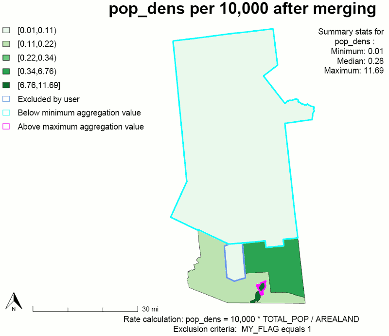
Map: Choropleth of Rate for Aggregated Areas

About this step

This step calls the function plotGATmaps() to draw the map.

File saving section

This section contains the file saving steps.

Step 21. Save maps and settings

Progress Bar: Save a PDF of the maps

In this section, all maps are saved to a PDF file, with one map per page, in the same folder as the aggregated shapefile. The same save filename is used with “plots” at the end.

An Rdata file is also saved. This file includes all settings in R format, which can be opened in R or run through GAT a second time. If you want to use the Rdata file to re-run GAT, use this code and change myfilepath to the location and name of your Rdata file:

myfilepath <- "C:/users/ajs/mygatfilesettings.Rdata"
gatpkg::runGATprogram(settings = myfilepath)

File saved to the save folder if you followed the vignette:

• hftown_agg6k15k_popwtplots.pdf (containing 5 maps)
• hftown_agg6k15k_popwtsettings.Rdata

Step 22. Save original shapefile

Progress Bar: Save the Original Shapefile

The purpose of saving this shapefile is to provide a key/crosswalk (GATid) identifying which aggregated area each original area fell inside when aggregated. The GATflag variable flags areas that were excluded from aggregation or generated warnings in the log:

• value = 0: no flag
• value = 1: area excluded based on exclusion criteria
• value = 5: area excluded because value of aggregation variable exceeded maximum value

The original shapefile is saved with the following changes:

• It is renamed to match the save filename you selected with “in” at the end and saved in the same folder as the aggregated shapefile.
• The variables GATid and GATflag are appended to its dataframe.

Files saved to the save folder if you followed the vignette:

• hftown_agg6k15k_popwtin.dbf
• hftown_agg6k15k_popwtin.prj
• hftown_agg6k15k_popwtin.shp
• hftown_agg6k15k_popwtin.shx

Step 23. Save aggregated shapefile

Progress Bar: Save the Aggregated Shapefile

In this section, the aggregated shapefile is saved. It includes all of the variables in the original shapefile with these changes:

• For categorical variables, the first option was selected for each merge.
• For numeric variables, the values were summed unless the variables represented latitude or longitude (or x and y), in which case they were averaged.

Additional variables created as part of the aggregation process and included in the shapefile’s database:

• GATx: longitude of area centroid (geographic unless population weighting was selected)
• GATy: latitude of area centroid (geographic unless population weighting was selected)
• GATcratio: compactness ratio for the area
• GATnumIDs: The number of original areas that were merged into each aggregated area
• GATflag: flag of areas that were excluded from aggregation or generated warnings in the log
  • value = 0: no flag
  • value = 1: area excluded based on exclusion criteria
  • value = 5: area excluded because value of aggregation variable exceeded maximum value
  • value = 10: value of area’s aggregation variable is below minimum value, but no other areas are eligible for further aggregation

Files saved to the save folder if you followed the vignette:

• hftown_agg6k15k_popwt.dbf
• hftown_agg6k15k_popwt.prj
• hftown_agg6k15k_popwt.shp
• hftown_agg6k15k_popwt.shx

Step 24. Save KML file

Progress Bar: Save the KML File

In this step, nothing happens if you are following the vignette and selected no when asked if you wanted to save a KML file. If you had selected yes, a KML file would be created in this step that could then be opened in Google Earth.

Files saved to the save folder, if “Yes” was selected in Step 9:

• hftown_agg6k15k_popwt.kml

Step 25. Save log

Progress Bar: Save the Log of Your Run

In this step, a text file is saved that includes all of your settings, basic information on data distributions for the aggregation variable(s), and warnings regarding possible issues with the aggregation.

Files saved to the save folder if you followed the vignette:

• hftown_agg6k15k_popwt.log

GAT is finished, now what?

Where to find your files

All files are saved to the save folder you selected. The log file contains a partial list of files created. The R console will display a full list of all files created and their location when the aggregation is complete, which will look something like this:

The following files have been written to the folder
C:/Users/ajs11/Documents/GAT:
hftown_agg6k15k_popwt.dbf
hftown_agg6k15k_popwt.prj
hftown_agg6k15k_popwt.shp
hftown_agg6k15k_popwt.shx
hftown_agg6k15k_popwtin.dbf
hftown_agg6k15k_popwtin.prj
hftown_agg6k15k_popwtin.shp
hftown_agg6k15k_popwtin.shx
hftown_agg6k15k_popwtplots.pdf
hftown_agg6k15k_popwt.log
hftown_agg6k15k_popwtsettings.Rdata

See the log file for more details.

How to use your files

• Shapefiles (*.shp): Open in ArcGIS, QGIS, or similar GIS software.
• KML file: Open in Google Earth desktop or online.
• PDF file: Open in any PDF reader.
• Log file: Open in any text editor, such as Notepad++.
• R data file (*.Rdata): Open in R using the format load("C:/filepath/settings.Rdata").